On the Problem of Time in Quantum Mechanics

Executive Summary

One of the overarching issues plaguing quantum mechanics is that there is no time observable, despite our ability to seemingly measure time. This is due to our treatment of time as an external backdrop in quantum mechanics, as opposed to the internal and relative time of Einstein’s theories of relativity. The discrepancy between how we treat time in quantum mechanics and relativity contributes towards our inability to reconcile the two disciplines and construct a theory of quantum gravity. Furthermore, a constraint in the form of the Wheeler-DeWitt (WDW) equation derived from combining aspects of general relativity and quantum mechanics begets a further problem regarding time; that the universe should be static, despite our observations of time-dependence.

This dissertation explores the Page and Wootters (PW) conditional probability approach to addressing the problem of time in quantum mechanics. By first explaining the fundamental concepts of quantum mechanics used in the PW approach and covering some of the issues that time faces in quantum mechanics, I lay the groundwork for understanding the PW approach and its significance. PW’s goal was to find an internal time in quantum mechanics to explain how the universe displays dynamical evolution despite the WDW equation enforcing an overall static state, as well as constructing a time observable that is consistent with how time is treated in relativity. This would allow for a definitive step forward in unifying quantum mechanics with general relativity.

They stated that the reason the WDW equation suggests we should see a static universe is because the constraint uses an external coordinate time. Therefore, while an observer with access to the external time would see the system as static, an observer who instead has access to the internal time should see a dynamical system. They used a mechanism of variable dependence between entangled yet non-interacting subsystems of a closed system to derive this dynamical behaviour. The PW approach is best illustrated by Moreva et al in a photon experiment which I cover towards the end of the dissertation. In this experiment, entangled photons are observed by an internal observer entangled with the system and with access to the internal clock time, and an external observer with access to abstract coordinate time and who is as such not entangled with the photon system.

The variable dependence mechanism utilised in the PW approach offers a promising explanation for the origins of time-dependence in the universe. Aiming to construct a time observable from a clock subsystem, it is, however, unsuccessful in constructing a time operator. The results of the photon experiment demonstrate a successful application of the PW approach; the internal observer noted an evolution of one photon with respect to the other, and the external observer noted an overall static state of the system.

A solution to the problem of time is important in order to reconcile quantum mechanics and general relativity, and in doing so provide a more cohesive theory of the universe and how it and everything within it works. Although issues remain within it and more work needs to be done to resolve them, the PW approach provides an excellent and innovative foundation for a solution to the problem of time in quantum mechanics, and should be further developed.

Introduction

Einstein’s theory of general relativity revolutionised the way we think about space and time on a grand scale. We learnt that space and time are joined together in the inseparable fabric of spacetime, and that neither space nor time are absolute, but rather are relative to the observer. The incredible explanatory powers of general relativity should be applicable to the subatomic scale at which quantum mechanics operates. Quantum mechanics provided enlightenment on the fundamental behaviour of particles such as electrons and quarks, as well as photons. The hope with quantum mechanics was that by describing the behaviour of such fundamental building blocks of reality, macro systems could also be described in these terms. However, a problem arises when trying to combine general relativity with quantum physics: they appear to be irreconcilable.

Relativity treats time as an intrinsic or internal measure, meaning that as a theory it is background-independent. Furthermore, general relativity treats space and time equally, as both space and time form as part of the same fabric. One major problem that arises when trying to fit general relativity with quantum mechanics is that, on a quantum scale, we treat time not as relative, but as a backdrop against which quantum events unfold uniformly- as an external parameter which is therefore not equal to space. But how can this be? Either time must progress at the same rate for quantum events and, therefore, all macro systems, or time must be relative not only for macro systems but also at quantum scales, requiring quantum frames of reference [1, 2]. A result of treating time as an external parameter in quantum mechanics is a lack of a time observable. This is troubling because we seemingly are able to measure time, so a mathematical equivalent to this measurement should exist [3].

The problem of time in quantum mechanics is really a collection of problems involving time [4], including issues such as the lack of a time observable and the discrepancy between the treatment of time in relativity and quantum mechanics, as well as the problem of time from the Wheeler-DeWitt (WDW) equation which I cover in Sec. 3.4. To have any hope of unifying general relativity with quantum mechanics, a step in the right direction would be to ensure that time is treated equally in both [5]. This means that for time to be an observable, it must be an internal measure as opposed to the external one we currently treat it as in the Schrodinger equation [3].

The three major approaches to solving the problem of time have been outlined by Kuchar [6, p.178]: finding an internal time in general relativity before quantisation, finding a time within the Wheeler-DeWitt equation or interpreting it in a dynamical way, and interpreting the Wheeler-DeWitt equation without requiring time and thus “treating time within our present-day theories, general relativity and quantum theory, as an approximate concept” [4, p.147]. Isham notes that a clear distinction should generally not be made between the latter two approaches [4, p.150].

Within general relativity, time is not absolute, and as such there is no standard time variable. Instead, there is the notion of ‘proper time’; the time measured by a clock along the particular worldline it finds itself on describing local systems along that worldline, where a worldline is simply the path that an object is moving along in spacetime. The proper time of a local system measures time for that system in the same way in which absolute Newtonian time measures time for classical systems. Such a formulation of time is necessary in general relativity because there is no one true flow of time, but rather time is relative to each observer or reference frame. For example, if one were to put a clock at sea level on earth and another clock orbiting the earth in space and then measure on each clock the time taken for the orbiting clock to orbit earth once, each clock would have a different reading. Both clocks were measuring their own proper time, which is relative to the other clock, and is parameterised by an arbitrarily chosen time, t. As such, it does not make sense to ask which of the two clocks has the correct time- which one was measuring the true time- because such a notion doesn’t exist; both were measuring their own ‘true’ (proper) times. Therefore, there can be no absolute time variable within general relativity. Finding an internal time within general relativity in the sense mentioned above means finding a time observable, which cannot be the proper time, before any quantisation. However, this is a burdensome task and has not been accomplished thus far [4], as it comes with its own set of problems, such as the problem of global time or the problem of many-fingered time evolution [6].

This brings us to the Wheeler-DeWitt equation, which I will explain further in Sec. 3.4. For now, it is worth knowing that there is no time within it and as such it describes the universe as static, which is why certain approaches need to be taken to either recover time from it or formulate a way in which quantum mechanics can work without time being fundamental to it. The latter is what the third approach involves; interpreting quantum mechanics in a completely timeless way and holding that fundamentally there is no time. Such is the view Rovelli discusses, in which he proposes that although on a subatomic level time doesn’t exist, it can be approximately reconstructed for classical purposes [7]. The obvious problem with the timeless approach is that we observe time passing all the time- everything is described as evolving with respect to time, so if time doesn’t exist at the quantum level, them from where or what do we reconstruct a time? Rovelli’s answer is that this comes from our psychology perceiving the thermodynamic arrow of time [7]. However, in explaining more recent interpretations of the concepts within thermodynamics and general relativity, Barbour has shown that Rovelli’s ideas depend upon the older versions of the theories which we now know to be incomplete, and so the ideas don’t stand up as well as he may have thought [8]. Other problems with the idea of a timeless quantum mechanics have been reviewed by Smolin [9]. As it stands, I am of the opinion that there are too many issues with the timeless approach to solving the problem of time, which is why in this dissertation I am going to be focusing on the second approach: that of finding a time within the Wheeler-DeWitt equation.

It is my opinion that Rovelli is indeed correct when he stated that mechanics is “a theory of relations between variables” [7, p.1] and that “what we can observe are the system’s quantities ai and the clock’s quantity β, and their relative evolution” [7, p.3], but that this doesn’t necessarily have to be the end. Instead of interpreting these ideas to mean that time does not exist at all and giving up on finding a time observable, I believe that finding a time observable suitable for use in a theory of quantum gravity is still a possibility which should be pursued, and that a promising way in which to do it is precisely that of measuring the relative evolution between variables.

When finding an approach to redefining time in quantum mechanics and ensuring that it is treated in the same way as space, two methods can be taken. Because time is not an observable and space is, the methods consist in either promoting time to the status of observable, or demoting space to a parameter like time, so that it is not an observable either [10]. The conditional probability method proposed by Page and Wootters (PW) follows the first method. They promote all the variables in the system to the status of observable and then choose one of them to be the quantum clock [11]. I am following this approach because the problem of time in quantum mechanics involves both that time is treated as an external parameter rather than an internal variable and that there is no time observable, and the PW approach, if successful, resolves both of these issues. Furthermore, the PW approach explains how it is that we observe dynamical evolution while the universe still obeys the WDW constraint.

This dissertation is structured as follows: after providing explanations of the basic quantum mechanics concepts needed to understand the PW solution to the problem of time in quantum mechanics, I outline what a time operator would require, as well as objections to the construction of such an operator, before explaining the problem of time arising from the Wheeler-DeWitt equation. I subsequently delineate the PW approach [5] to solving the problem of time that arises from the Wheeler-DeWitt equation, explaining the mechanism behind the PW approach and its successes, before focusing on an experiment conducted by Moreva et al [12] based on the PW approach. The final section discusses the PW approach as it stands currently, as well as outlining the objections and further revisions made to the approach.

Quantum Mechanics

In this section, I give an overview of quantum mechanics to lay out the fundamental concepts needed for explaining the Page and Wootters approach to constructing a time observable and obtaining time evolution.

State vectors and the Wavefunction

A state vector, $|\Psi \rangle$, is a vector that represents the state a quantum system is in, containing all the possible information about the system. It exists in an infinite-dimensional mathematical space called a Hilbert space, and as such is a general representation of the state of the system, being more broadly defined. A wavefunction is a state vector projected onto a particular basis, a common one being the position basis. It exists in configuration space rather than Hilbert space, a 3N-dimensional space that encodes the locations of particles in points within it.

The relation between the state vector and wavefunction is demonstrated by

\begin{equation} \psi(x)=\langle x | \psi \rangle \end{equation}

where $\langle x | \psi \rangle$ denotes the inner product between the position bra vector and the state ket vector, mapping the state vector to the position representation.

Alternatively, the state vector is given by

\begin{equation} | \psi \rangle = \int_{-\infty}^{+\infty} \psi(x)|x\rangle \,dx \end{equation}

where the product of the wavefunction in the position representation, $\psi(x)$, and the position ket vector, $|x\rangle$, are integrated over all space.

Operators and Observables

In quantum mechanics, an operator is a mathematical object or function that acts on a wavefunction, mapping it to a new wavefunction. This new wavefunction demonstrates that the system has changed in some way, such as if it is evolving with time. An operator can also be thought of as mapping the state vector of a system onto a different state vector within the Hilbert space.

An operator is given generally in Dirac notation by

\begin{equation} \hat{O} = |o\rangle \langle o| . \end{equation}

For example, the position operator is given by

\begin{equation} \hat{x} = \int_{-\infty}^{+\infty} |x\rangle x \langle x| \,dx \end{equation}

with an integral over $dx$ because it is easier to assume that space is continuous.

An observable in quantum mechanics is a physical property of a system that can be measured, such as position, momentum, or energy. An observable is an operator that is also self-adjoint or Hermitian, and so its eigenvalues are real. For example, the position operator $\hat{x}$ is an observable which multiplies a wavefunction by x, thereby mapping it onto the x coordinate axis. The eigenvalues of an observable are the possible measurement outcomes for that observable.

The Schrodinger Equation

The evolution through time and space of a wavefunction of a quantum system is determined by the time-dependent Schrodinger equation

\begin{equation} \label{SE} i{\hbar}\frac{\partial}{\partial t}|\Psi \rangle = \hat{H}|\Psi \rangle \end{equation}

where i is the imaginary number given by the square root of −1, \({\hbar}\) is Planck’s constant divided by \(2\pi\), t is the external time, \(\hat{H}\) is the Hamiltonian observable and \(\|\Psi \rangle\) is the state vector of the quantum system.

The Hamiltonian, consisting of the kinetic energy operator $\hat{T}$ and the potential energy operator $\hat{V}$ in the form \(\hat{H}=\hat{T}+\hat{V}\) corresponds to the total energy of a system. It forms as part of Eq. (5) because the evolution of a quantum system through time and space depends on its total energy.

The Schrodinger equation can be written as an eigenvalue equation

\begin{equation} \hat{H}|\Psi \rangle = E|\Psi \rangle \end{equation}

where the state vector $|\Psi \rangle$ is the eigenvector or eigenstate, and the energy E is the eigen value. Solving this eigenvalue equation yields the possible energies of the system and the corresponding state the system can be in for each possible energy.

Due to the linearity of the Schrodinger equation, the state of a system can be represented as a superposition of states

\begin{equation} |\nu \rangle = \sum_{n}^{} \alpha_n |\nu_n \rangle = \sum_{n}^{} |\nu_n \rangle \langle \nu_n | \nu \rangle . \end{equation}

Any linear combination of state vectors \(\|\nu_n \rangle\) can be summed to form a new state vector \(\|\nu \rangle\), with each constituent vector having its own weighting denoted by a coefficient, $a_n$ or \(\langle \nu_n \| \nu \rangle\), which may be complex. Such a linear combination represents the state of a system before measurement. The magnitude squared of the complex coefficient denotes the probability of the system collapsing to that state, and the sum of the magnitude squared of the coefficients is 1 when the states are normalised.

Measurement and Expectation Values

A superposition of eigenstates also means a superposition of eigenvalues. Upon measurement, the system, previously composed of a superposition of states, ‘collapses’ to one of the eigenstates, which is how we obtain a real value from the measurement.

Projection operators are used to project a state into a different basis. Using a projection operator is the mathematical equivalent of performing a measurement on a system. It projects the state onto the subspace given by the projection operator, meaning that only the parts of the state originally within that subspace remain.

As it is an operator, it is defined in the same way as any operator. An example of a projection operator might be

\begin{equation} \hat{\mathbb{P}}_a = |a \rangle \langle a| \end{equation}

which when acting on a state would project it onto the subspace defined by |a⟩.

The probability of obtaining a certain eigenvalue when performing a measurement on a system is given by

\begin{equation} {|\langle o|\psi \rangle |}^2. \end{equation}

For example, the probability of finding a particle in a given eigenstate of position is \({\|\langle x\|\psi \rangle \|}^2\)

The probability of finding a particle between x and x + dx, or the probability density, is given by \({\|\psi (x)\|}^2\) Therefore, to calculate the average value of a system, termed the expectation value, one integrates over the product between the probability density and the observable

\begin{equation} \langle \psi |\hat{O}| \psi \rangle = \int_{-\infty}^{+\infty} {| \psi (o) |}^2 \cdot o \,do \end{equation}

where $\hat{O}$ represents any operator. For example, to calculate the position expectation value one would do \(\langle \psi \| \hat{X} \| \psi \rangle\) which corresponds to:

\[\int_{-\infty}^{+\infty} {\psi (x)}^* x \psi (x) \,dx\]

Entanglement

Two particles are entangled when their own states are dependent upon the state of the other particle and cannot be written in terms independent from the other particle until measurement. Before measurement, it is only possible to write the overall state of the two particles. The state of one is not separable from this overall state and is not knowable.

To demonstrate this, an example of a non-entangled, separable state is

\begin{equation} |\Psi \rangle = \frac{1}{\sqrt{2}} (|00\rangle + |10\rangle). \end{equation}

This state is not entangled because the state vectors are factorable. The state can be written as

\begin{equation} |\Psi \rangle = \frac{1}{\sqrt{2}} (|0\rangle + |1\rangle) \otimes |0\rangle \end{equation}

where the part in the parentheses is a superposition of two states for one particle and the other particle is in the state |0⟩.

An entangled state is not factorable in this way. An example of a maximally entangled state, or Bell state, is

\begin{equation} |\Psi \rangle = \frac{1}{\sqrt{2}} (|01\rangle + |10\rangle). \end{equation}

This cannot be factored into the states of two particles and is therefore an entangled state.

Density Matrices

Density matrices are an alternative way to represent the state of a system which, like the state vector, contain all the information about the system. A density matrix for a pure system is that system’s projection operator, defined as

\begin{equation} \rho = \sum_{i}^{} c_i |\phi_i \rangle \langle \phi_i | = |\phi \rangle \langle \phi | \end{equation}

where $c_i$ is the coefficient giving the weighting for each particular state, $\phi_i$. For a mixed state, the sum is still over all the possible states the system could be in, but is not simply a single \(\|\phi \rangle \langle \phi \|\) term.

Density matrices are especially useful for representing entangled systems, which are an example of a pure state comprised of two or more mixed states. While it is possible to know the state vector for a pure state, for mixed states this is not possible- as with entanglement, in which it is not possible to know the states of component parts of the system until a measurement is performed. However, the density matrix representing a mixed state can be known. Therefore, when performing calculations on entangled systems such as for calculating the individual states in the system, this must be done using the density matrix.

To form a density matrix for a system comprised of multiple smaller subsystems, a tensor product is performed between the density matrices for the smaller subsystems. A density matrix for subsystems and A and B would be

\begin{equation} \rho_{AB} = \sum_{j}^{} k_j \cdot \rho_{Aj} \otimes \rho_{Bj} \end{equation}

where $k_j$ is a constant weighting each tensor product.

Therefore, to obtain the density matrices for one of the smaller subsystems from the overall system, a partial trace must be performed.

\begin{equation} \rho_A = Tr_B[\rho_{AB}] = \sum_{r}^{} \langle r | \rho_{AB} | r \rangle \end{equation}

shows that to obtain the reduced density matrix for subsystem A, a partial trace over the composite density matrix needs to be performed. This is to ‘trace out’ particle B and obtain the reduced density matrix for particle A. If the resulting density matrix is for a mixed state then the two particles are entangled. A is a mixed state if the trace of the square of the reduced density matrix for A is less than 1.

Density matrices can also be used to calculate expectation values for a system,

\begin{equation} \langle A \rangle = Tr(A\rho). \end{equation}

This works because the diagonal elements of a density matrix are the probabilities for obtaining different eigenvalues, so the sum of the product between each diagonal element with its corresponding eigenvalue gives the average value.

Commutation Relations and Uncertainty Relations

Two operators commute when the relation

\begin{equation} [\hat{A}, \hat{B}]=0 \end{equation}

is satisfied, where \([\hat{A}, \hat{B}]= \hat{A}\hat{B} - \hat{B}\hat{A}\) and they do not commute when

\begin{equation} [\hat{A}, \hat{B}] \neq 0 . \end{equation}

Observables are compatible when their corresponding operators commute and are incompatible when they do not. If two operators commute, they share a complete set of eigenvectors, which means that it is possible to construct a shared simultaneous basis of eigenstates. This means that for any commuting operators, when a measurement for an observable is made on a particle and its wavefunction ‘collapses’ to an eigenstate, since this eigenstate is also an eigenstate for the commuting operator, one can obtain eigenvectors for both the operators simultaneously. That is to say, one can perform a simultaneous measurement for both the observables and obtain definite states for both simultaneously. For two operators that do not commute, it is not possible to perform simultaneous measurements of the two and obtain a definite state for each. Such observables whose operators do not commute are also known as complementary variables. This property of non-commutable operators is what leads to the uncertainty relations. For example, the canonical commutation relation

\begin{equation} [\hat{x}, \hat{p}] = i\hbar \end{equation}

leads to the Heisenberg uncertainty principle for position and momentum

\begin{equation} \Delta x \cdot \Delta p \geq \frac{\hbar}{2} \end{equation}

which states that the product between the uncertainty in the position and the uncertainty in the momentum, where the uncertainty is given by the standard deviation, cannot be less than Planck’s constant over \(4\pi\)

If an observable commutes with the Hamiltonian of the system, then the observable is a conserved quantity, and so does not evolve with time. This is demonstrated by first writing out an arbitrary state for an observable $\hat{O}$ which commutes with the Hamiltonian

\begin{equation} |\psi (t=0) \rangle = \sum_{i}^{} c_i |\lambda_i \rangle \end{equation}

where $c_i$ is a constant such that \({\|c_i\|}^2\) gives the probability of having the system in the eigenstate \(\|\lambda_i \rangle\).

Because we have that the observable \(\hat{O}\) commutes with the Hamiltonian, they necessarily share a common set of eigenstates. This means that the state \(\|\psi (t=0) \rangle\) representing the linear combination for \(\hat{O}\) must also be the linear combination for the energy eigenstates, and so

\begin{equation} | \psi (t=0) \rangle = \sum_{i}^{} c_i e^{-i E_t t/\hbar} |\lambda_i \rangle . \end{equation}

Therefore, the probabilities will be \({\|c_i e^{-i E_t t/\hbar}\|}^2\) resulting in the exponent term becoming 1 and the probability being time-independent.

Time in Quantum Mechanics

In this section, I demonstrate how the treatment of time in quantum mechanics results in an uncertainty relation between energy and time that does not have the same meaning as a canonically conjugate pair. I outline Pauli’s objection as to why there can be no time operator, as well as explaining how a time operator must be structured. Finally, I outline the Wheeler-DeWitt equation along with its implications for time evolution within the universe, resulting in the problem of time from the Wheeler-DeWitt equation.

Time Commutation Relation

Another relation between two complementary variables is the energy and time uncertainty relation

\begin{equation} \Delta E \cdot \Delta t \geq \frac{\hbar}{2} . \end{equation}

The relation states that the product between the energy of a particle in a state and the time it takes for the system to change considerably (i.e. to evolve to an orthogonal state) must be greater than or equal to Planck’s constant divided by \(4 \pi\) Instead of $\Delta t$ representing the standard deviation of time measurements, it is the time taken for the expectation value of the energy observable to change by one standard deviation. This relation is fundamentally different from the position and momentum uncertainty relation because the time here is not a physical quantity, since there is no time observable.

If the time in the uncertainty relation were instead a time observable and if instead of the energy one were to use the Hamiltonian H such that the uncertainty relation read:

\[\Delta H \cdot \Delta T \geq \frac{\hbar}{2}\]

the commutation relation giving rise to such an uncertainty relation would be

\begin{equation} [\hat{H}, \hat{T}] = i\hbar . \end{equation}

However, in the next section I cover the argument against such a commutation relation being possible.

Objections Against Time Operators

The Stone-von Neumann theorem states that any pair of observables that are canonically conjugate, such that \([\hat{A}, \hat{B}] = i\hbar\) have all the same properties as the canonically conjugate Schrodinger pair [3]. One such property is that both the operators must be unbounded from both above and below. However, the Hamiltonian is bounded from below, meaning that it can’t form a canonically conjugate pair with another operator. Because the Schrodinger equation is the generator of time translations, the time observable would be the variable canonically conjugate to the Hamiltonian. However, since the Hamiltonian cannot form a canonically conjugate pair, there cannot be an operator that fulfils the necessary requirements for being a time operator.

A consequence of the Stone-von Neumann theorem is Pauli’s objection to there being a time operator. If the commutation relation of \([\hat{H}, \hat{T}] = i\hbar\) holds, the Hamiltonian and time observable must share a common spectrum of eigenvalues [13]. However, because the Hamiltonian has a lower bound while time is typically unbounded, they would not share all the same eigenvalues. Therefore, the self-adjoint time operator is not possible.

Time Operator

If a time operator were to be formed, it would need to be defined at one position in space: because we have position as dependent on time, x(t), which gives the location at a particular time, the reverse must also be true- the time must be given at a particular location, t(x).

Therefore, the time operator must be of the form

\begin{equation} T(x_0)= \int_{-\infty}^{+\infty} t|x_0, t \rangle \langle x_0, t| \,dt \end{equation}

giving the time at the location $x_0$.

A state vector in space and time would have to be defined as

\begin{equation} |\phi \rangle = \int_{-\infty}^{+\infty} \,dx \int_{-\infty}^{+\infty} \,dt \phi (x, t) |x, t \rangle . \end{equation}

This is summing over all of space and time and so effectively would require space and time to be treated equally. Instead of a snapshot of the state at one time for all of space, it is more like a film detailing the state in space through time. This necessarily requires the Wheeler-Dewitt equation constraint [3].

An interesting consequence of having a time operator would be time eigenvalues and eigenstates, resulting in a superposition of different times.

The Problem of Time from the Wheeler-DeWitt Equation

In this subsection I give a layout of the Wheeler-DeWitt (WDW) equation and its implications in the search for quantum time by illustrating the problem of time that emerges from it, as well as the consequences this has for a theory of quantum gravity.

The WDW equation,

\begin{equation} \hat{H}(x)|\Phi \rangle = 0 \end{equation}

is a constraint on the state vector of the universe which comes about from quantising general relativity and having a state vector which treats space and time equally [12]. The left-hand side of the Wheeler-DeWitt equation is the Hamiltonian operator acting on the state vector of the entire universe. Because it equals 0, this means that the universe is in an eigenstate of its Hamiltonian with eigenvalue zero.

Because the WDW equation is a constraint on the Hamiltonian in quantised general relativity, it is both relativistic and quantum. This is why the equation is seen as an equation of quantum gravity, and why interpreting it is important.

Furthermore, unlike the Schrodinger equation, the WDW equation does not include a time because in general relativity there is no absolute time; time in general relativity is treated as a dimension or coordinate, and the time measured by an observer is a relative internal time. This is confusing when considering quantum mechanics because the wave function should describe the state of the universe at a particular time, and the Hamiltonian should tell us the evolution of the system with time. But the WDW equation, the constraint on the Hamiltonian, does not here describe the evolution of the system with time. The system described here is the entire universe, so what the WDW equation says is that the universe is not evolving with time but rather is static.

This result is contradictory to what we observe every day: a dynamical universe that changes with time. Attempts to find a time within the WDW equation stem from this contradiction, and a successful solution would explain why we observe the universe as non-static. This is one form of what the problem of time becomes: explaining how within the universe we observe temporal phenomena when the WDW equation predicts a stationary universe [1].

The Page and Wootters Approach

Page and Wootters proposed that we use an external time in quantum mechanics that is not observable, and that instead of this we should use an internal time [5]. They aimed to find a time-dependence and a time observable despite all observables and the universe needing to be static. I here give an overview of the original formulation of the PW approach, and briefly cover the reformulations in Sec. 6. This is to better understand how the approach aims to solve the problem of time, as well as to lay the foundations for the experiment conducted by Moreva et al.

What PW proposed is that the WDW equation declares the universe as static because it is, but only with respect to an external coordinate time, whereas the time evolution we see within the universe is due to a dependence on an internal, physical time. We see the universe as dynamical because we are within it and as such entangled with it, but if a hypothetical external observer (which, as far as we know, it is impossible to have) were to measure the overall state of the universe via the universal wavefunction and compare it to a background coordinate flow of time, they would find that the state is static and so obeys the WDW equation.

As well as the WDW equation constraint on the energy of the universe, Page and Wootters found that there must be a superselection rule for “energy… coupled to a long-range gravitational field” [5, p.2885], resulting in the fact that for an operator to be an observable it must commute with the Hamiltonian. However, this means that such observables must be stationary, meaning they have no time-dependence. This is a problem, as we clearly do measure observables as having a time-dependence in the universe. I cover the issues resulting from this in Sec. 6.

Within the PW approach, the overall subsystem is divided into two subsystems: one acting as a clock, and one consisting of the rest of the system. PW state that the time dependence we observe is due to the dependence on the clock subsystem of the subsystem constituted by the rest of the system, or ‘rest subsystem’. An important point to note is that this dependence works both ways. In effect, it makes no difference which subsystem one chooses to act as the clock, as the two subsystems can be interchanged in the equations so that each is dependent on the other. This concept mirrors how time works in relativity, with time being relative to each frame of reference and no frame of reference having the one true time.

Variable Dependence

Here I explain how it is that the rest subsystem is dependent on the clock subsystem, resulting in dynamical evolution.

The variable dependence in the PW approach relies upon Everett’s concept of relative states, the basic idea of which is that when two subsystems of an isolated system interact, they become entangled so that each one’s state can only be described in terms of the other’s state [14]. However, this reliance upon Everett’s concept of relative states does not require that we adopt the Everettian interpretation of quantum mechanics. It is possible to have the concept of relative states without necessarily having to make the ontological claim that the wavefunction is real, therefore preventing an endless branching of worlds upon effective wavefunction collapse [1]. However, like in Everett’s relative state theory, the universal wavefunction within the PW approach does not collapse upon measurement [1].

The state of the overall system is given by the entangled global stationary state [15]

\begin{equation} |\Phi \rangle = \sum_{t}^{} c_t |\phi (t) \rangle_c \otimes |\phi_t \rangle_r \end{equation}

where \(c_t\) are constants such that \(c_t \neq 0\), \(\| \psi (t) \rangle_c\) are the eigenstates of the clock observable,
\(\|\phi_t\rangle_r\) are the states of the rest subsystem conditioned to the clock state being \(\| \psi (t) \rangle_c\), and \(\|\Phi\rangle \in \mathcal{H} = \hat{\mathcal{H}}_c \otimes \hat{\mathcal{H}}_r\). Thus, to obtain the values for the rest subsystem, a partial trace will need to be performed.

The state of the rest subsystem is defined relative to the state of the clock subsystem [15]

\begin{equation} \rho_t^{(r)}= \frac{Tr_c[P_t^{(c)}\rho]}{Tr[P_t^{(c)}\rho]} = |\phi_t \rangle \langle \phi_t | \end{equation}

where \(\rho = \|\Phi \rangle \langle \Phi \|\) is the density matrix operator with \(\|\Phi \rangle\) being the state defined above in Eq. (29), and \(P_t^{(c)} = \|\psi (t)\rangle \langle \psi (t)\|\) is the “projector on a certain time state in the clock subspace” [15, p.9], also called the time observable. This follows Everett’s relative state equation for describing two interdependent systems.

The numerator in this equation is performing a partial trace over the clock states in the density matrix, thus tracing out the clock components from the density matrix. The denominator is performing a trace over the full density matrix of the entangled system, and together they define the state of the rest subsystem relative to the clock subsystem in the form of a reduced density matrix.

Conditional Probability and Expectation Values

Because the two subsystems are entangled, the probabilities associated with one are de pendent on the other and cannot be calculated without the other. The probabilities must be calculated as conditional probabilities. The probability of obtaining a value a for an observable $\hat{A}$ on a subspace at a time t on the clock subsystem C is calculated given that the clock subsystem has the time t [15],

\begin{equation} P(A=a|C=t)= \frac{P(A=a, C=t)}{P(C=t)}. \end{equation}

The conditional probabilities demonstrate the dependence of the rest subsystem on the clock subsystem, thus demonstrating the ‘time-dependence’ of the rest subsystem. This is because the probabilities for obtaining a value for the rest subsystem change with a changing value of the clock subsystem. The other way in which this is demonstrated is by the conditional expectation values [5].

For a dynamical variable A which is dependent on the clock reading t with projection operator $P_t^{(c)}$, the conditional expectation value for A is

\begin{equation} E(A|t)=\frac{Tr(\overline{P_t^{(c)} A P_t^{(c)}}\rho)}{Tr(\overline{P_t^{(c)}}\rho)} \end{equation}

in which $\rho$ is again the density operator of the whole system. The averaging is necessary in order to ‘average out’ the unobservable external time so that the quantities $\overline{P_t^{(c)}}$ and $\overline{P_t^{(c)} A P_t^{(c)}}$ are static and therefore observable. This is due to the superselection rule which states that any observables must be static. The density matrix $\rho$ is not averaged over, but were we to replace $\rho$ with its corresponding stationary state $\overline{\rho}$ (the time average of $e^{-iHt}\rho e^{iHt}$), the conditional expectation values would yield the same results [5].

If, instead of a dynamical variable A, we have A as a projection operator $P_\alpha$ onto an eigenspace $\alpha$, the conditional expectation value is defined as

\begin{equation} E(P_\alpha |t) = P(\alpha | t) \end{equation}

which is the conditional probability as defined above in Eq. (31).

Obtaining Dynamical Evolution

A condition for the formulation of an internal clock time is that the system we are operating within must be a closed one, one in which all observers are within the system. The only truly closed system available to us is the universe [5], therefore allowing for application of this approach to the universe. In this section I detail how PW obtain time evolution within the universe despite the WDW equation enforcing an overall stationary state.

Importantly, because the conditional expectation values yield the same results whether we use $\rho$ or $\overline{\rho}$, there is no difference between the situation in which the universe is stationary, compared to the situation in which the universe is dynamical; they obtain the same dynamical behaviour either way [5]. We get the same result from evolution due to correlation with an overall stationary state as we do from evolution due to the equations of motion (SE) for an overall evolving state. Their approach essentially allows for the Wheeler-DeWitt constraint to be applied, meaning that the wavefunction of the universe is indeed static, while explaining time evolution within the universe in terms of entanglement. This dynamical evolution is shown in the following way:

A closed system denoted by $|\Phi \rangle$ is subdivided into two subsystems: the clock subsystem with Hamiltonian $H_c$, and the rest subsystem with Hamiltonian $H_r$. The total Hamiltonian for the system is then

\begin{equation} H = H_c \otimes \mathbb{I}_r + \mathbb{I}_c \otimes H_r \end{equation}

where $\mathbb{I}$ is the identity operator. This assumes one can neglect interaction between the two subsystems. The Hamiltonian is such because the Hilbert space for the system must be of the form $\mathcal{H} = \mathcal{H}_C \otimes \mathcal{H}_R$, where $\mathcal{H}_C$ is the Hilbert space for the clock subsystem spanned by the clock basis states and $\mathcal{H}_R$ is the Hilbert space for the rest subsystem spanned by its basis states. One can then obtain the regular quantum dynamics back for the rest subsystem by projecting the state of the system $|\Phi \rangle$ onto a state for the time t of the clock subsystem [12], where the state for the clock subsystem is $| \psi (t) \rangle_c = e^{-i H_c t/ \hbar}|\psi (0) \rangle_c$,

\begin{equation} |\phi (t) \rangle_r = {}_c\langle \psi (t) | \Phi \rangle = e^{-i H_r t / \hbar} |\phi (o) \rangle_r \end{equation}

which evolves in accordance with the equation of motion, the Schrodinger equation. This is how, even with a state that is static, one can derive dynamical evolution for subsystems of that state.

Perhaps assuming the clock subsystem is in this eigenstate is too strong, but Page and Wootters show that it is possible to make this assumption and then obtain dynamics [16].

Assumptions

Taking the universe to be static and timeless as per the WDW equation is only one of the conditions that the PW formalism assumes. It additionally requires good clocks to be possible, and that the entire universe is entangled with the clock subsystem [16]. The first of the two assumptions I will cover here is the assumption that a good clock is possible within the system. For the clock subsystem to make a good clock, the condition requires that the clock subsystem ideally does not interact at all with the rest of the universe, so that the Hamiltonian of the overall system can be written as the sum of the two subsystem Hamiltonians: $ H = H_c \otimes \mathbb{I}_r + \mathbb{I}_c \otimes H_r$.

Furthermore, an ideal clock would also be conjugate to the Hamiltonian, with the commutation relation $[\hat{H}, \hat{T}] = i\hbar$. However, despite T being merely the clock observable and not a time operator in this case, to circumvent Pauli’s objection the Hamiltonian still needs to be unbounded from below. Thus, the assumption is made that there exists a clock observable that can be conjugate to the Hamiltonian of the clock subsystem. How such a clock observable might be formulated in the PW formalism is discussed by Favalli and Smerzi [15].

The second assumption made is that the rest of the universe is entangled with the clock subsystem, as this is what results in dynamical evolution. This entanglement means that the universe must be represented by a state vector of the form as stated in Eq. (29).

Successes

Though the PW formalism has significant drawbacks that prevent it from being fully embraced as a leading theory of time, there are nevertheless a number of areas in which it succeeds. A prominent one is that a time observable is constructed. The time observable has eigenvalues and eigenstates of the clock subsystem, making it a suitable candidate for a quantum clock with quantised time eigenvalues. That these eigenvalues are quantised can be considered a further success, as quantum mechanics has been able to quantise almost every other possible observable, the notable exclusions being space and mass.

Additionally, the PW approach demonstrates some kind of time-dependence by showing that the rest subsystem has values and probabilities dependent on the clock subsystem and which evolve with respect to the clock subsystem. Whether this actually shows a time dependence is another matter, as this is a contentious issue- at least, a dependence between the two systems is shown. However, if one can take the clock subsystem as representing a real clock, then one may conclude that the rest subsystem does exhibit time-dependence.

Adopting the PW formalism means using an internal time much like the internal time of relativity. It is a significant success that the PW approach formulates a quantum time in the same way as relativity, albeit along quantum frames of reference. This is because it is helpful for constructing a theory of quantum gravity, as such a theory requires that time be treated equally in both relativity and quantum mechanics. Consequently, establishing an internal time in quantum mechanics is an important step towards this goal.

Finally, the obtention of dynamical evolution while still obeying the WDW constraint is perhaps the most important achievement of the PW approach, as this solves the problem of time arising from the WDW equation. This mechanism was masterfully demonstrated by Moreva et al in an experiment which I outline in the following section.

Experimental Illustration

An experiment that shows how the PW approach can be implemented was conducted by Moreva et al [12]. The experiment uses two entangled photons to demonstrate how time can emerge from the dependence between them while the overall entangled state remains static. After outlining the initial concepts and experimental setup, I describe the methods used and the results of the experiment.

Two static, entangled photons are polarized with either horizontal, $H$, or vertical, $V$ , polarization degrees of freedom. They are fired through various birefringent quartz plates to rotate their polarization, where the thickness of the plates gives the abstract coordinate time, as the polarization rotation is proportional to the thickness. One of the photons is the clock photon, with a polarization rate proportional to the amount of time it spends in between the birefringent plates, and the second photon is the one whose polarization evolves with respect to the clock photon and will be given in terms of the clock photon state. This is the photon shown to have a time-dependence.

Because the photons are entangled, their individual states are dependent on each other. The entangled state is given by

\begin{equation} | \Psi \rangle = \frac{1}{\sqrt{2}}(|H\rangle_c |V\rangle_r - |V\rangle_c |H\rangle_r) \end{equation}

where $H_c = H_r = i\hbar \omega (|H\rangle \langle V| - |V\rangle \langle H|)$ and where subscript $c$ denotes the clock photon and $r$ the second photon. Here, $\omega$ is the “polarization rotation rate of the quartz plate” [12, p.2], which means that the polarization of the photons is dependent on the time spent between the birefringent plates.

To demonstrate the PW approach, we must take the state of the entangled photons to obey the WDW constraint. That is, despite any time evolution observed of the system, the overall state of the system must remain static. Therefore, there must be two modes of observation carried out on the system: the observer mode, which measures the evolution of the second photon with respect to the clock photon to see how the components of the system evolve with respect to an internal time, and the super-observer mode, which measures the evolution of the global state of the system with respect to abstract coordinate time. The experimental setup for the two modes is shown in Fig. 1. In this way, it is possible to show how one can observe time evolution within a system while its overall state still obeys the WDW equation.

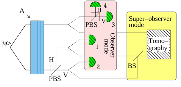Fig. 1: Experimental setup for Observer mode (a) and Super-observer mode (b), where A denotes the birefringent plates, PBS is a polarising beam splitter and BS is a beam splitter.

Observer Mode Method

The first mode of observation is the internal observer mode. This observer has knowledge of the polarization of both the clock photon and the other photon, and so is entangled with the two photon system. The internal observer does not have access to the abstract coordinate time– they do not have knowledge of the thickness of the birefringent plates. This is accomplished by using a difference plate thickness for each run of the experiment.

Once the photons are sent through the plates, the clock photon is sent at a polarizing beam splitter (PBS). The clock photon can only take one of two values, either horizontally polarized, $|H\rangle$, with detector 1 clicked and time $t = t_1$, or vertically polarized, $|V\rangle$, with detector 2 clicked and time $t = t_2$. The times follow the equation $t_2-t_1= \frac{\pi}{2\omega}$ which means that the polarization of the photon is flipped, or made orthogonal, in the time interval.

Detectors 3 and 4 are used to measure the polarization of the other photon; the photon is sent at another PBS, so detector 3 is activated for a vertically polarized photon and detector 4 for a horizontal polarization. Then, the conditional probabilities are calculated.

Observer Mode Results

The time-dependence of the second photon is expressed through the conditional probability of obtaining a certain result for the second photon given a certain time from the clock photon. For example, the conditional time-dependent probability that the second photon has vertical polarization is given by $p(t_1)=P_{(3|1)}$, the probability that detector 3 is activated given detector 1 has been activated, and $p(t_2)=P_{(3|2)}$, the probability that detector 3 has been activated given that detector 2 has been activated.

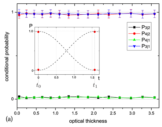Fig. 2: Experimental results for the Observer mode.

Fig. 2 shows that there is no dependence of the conditional probabilities on the abstract coordinate time represented by the thickness of the birefringent plates. Different plate thicknesses have no effect on the conditional probabilities obtained and thus on the time dependence of the second photon on the clock photon.

Super-Observer Mode Method

The super-observer has knowledge of the thickness of the birefringent plates and so has access to the abstract coordinate time. This is to test whether the overall state of the entangled system changes with respect to this abstract coordinate time.

However, the super-observer does not have access to the same information as the internal observer. The results of the second photon are given to the super-observer, but the results of the clock photon are first sent to a non-polarizing beam splitter (BS). This beam splitter is used to perform a quantum interference experiment, with the interference brought about by the beam splitter which will always polarize the light to one polarization. This erases the polarization information of the clock photon so that the super-observer does not have access to the internal clock time, subsequently becoming entangled with the clock.

The super-observer uses quantum state tomography to reconstruct the overall state of the system, and then compares this final state to the theoretical initial state of the system. Quantum state tomography is a process by which many projective measurements are made on the states to figure out a particular aspect of the state and therefore build up the overall state, for example through a density matrix.

Super-Observer Mode Results

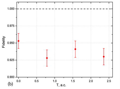Fig. 3: Experimental results for the Super-observer mode.

The conditional probabilities are calculated in the same way as for the internal observer. Here, the conditional probabilities calculated from the measurement results are compared with the conditional probabilities of the theoretical initial state. Fig. 3 shows the fidelity plotted as a function of the abstract coordinate time, where the fidelity is a measure of how much the initial and final states overlap and is given by $F= \langle \Psi_i | \Psi_f | \Psi_i \rangle$. As the graph shows, the fidelity is close to 1, meaning that the final state is close to the initial state, as expected of a static state.

Experimental Discussion

The experiment uses two modes: an internal observer, corresponding to a typical observer within the universe entangled with the clock subsystem, and an external observer, corresponding to what an observer outside the universe would measure (if such an observer were possible). The external observer is not entangled with the clock subsystem, but has access to the external flow of time instead.

Using these two modes of observation, Moreva et al implemented a successful application of the PW approach to demonstrate how a universe bound by the WDW constraint, which is therefore static, can be seen to evolve with time to observers within it. They illustrated this by showing that when an observer is entangled with a system of two photons, they can observe the evolution and therefore probabilities of the two photons as being dependent on each other and not on the abstract coordinate time. When an observer is not entangled with the system of two photons it is observed as remaining in a static state. This concept is then applied to larger subsystems within the universe to explain time evolution on larger scales.

Moreva et al also did a further experiment to show how the setup can be amended to construct a two-time propagator. This was to accommodate an objection to the PW approach which I discuss in the next section.

An important point to note about this experimental demonstration of the PW approach is that despite its sophistication, it is by no means a proof of the PW approach, but rather a very good demonstration of how the approach works.

Discussion and Conclusion

In this dissertation I first covered the foundational aspects of quantum mechanics used in the PW approach to understand the methods used in the approach. Following this, I explained some of the issues revolving around time in quantum mechanics, including the problem of time from the WDW equation.

The PW approach offers a solution to this problem of time, and is exemplified well by an experiment conducted by Moreva et al. The PW approach was conceived with the motivation of unifying quantum mechanics and general relativity by finding a time within quantum mechanics that is consistent with how time is treated in relativity. Page and Wootters went about this by proposing that an internal time on the quantum scale comes about due to the dependence of entangled subsystems on each other, and thus the dependence of the probabilities for the state of one subsystem on the state of the other subsystem, resulting in what is known as the conditional probability approach to time in quantum mechanics.

Despite using stationary observables, PW held that we can still observe change within the system and construct a time observable. PW attempted to show time evolution through promoting all the variables to the status of observable and then selecting one of these to act as the clock. However, an issue arises when considering which variable to use as the clock: if all the variables must commute with the Hamiltonian and are therefore static, none make particularly good candidates for a clock [11]– a variable that denotes temporal f low cannot be static.

PW attempted to resolve this using kinematical variables to act as the clock, as these necessarily are non-static and do not commute with the Hamiltonian [11]. Unfortunately, these kinematical variables exist in a kinematical Hilbert space which is unphysical [1] and so the variables are taken “out of the physical space” [17, p.74].

This resulted in Kuchar identifying that the construction of a two-time propagator is not possible: one can calculate conditional probabilities for $\hat{O}$ for a particle at a time $t$, but not the dynamical probability of finding the particle in the state $\hat{O}’$ at time $T > t$. [17]. That is, the propagators “do not propagate” [11, p.1]– they are “proportional to a Dirac delta function” [11, p.3].

In order to salvage the PW approach, Gambini et al [11] used Rovelli’s evolving constants of motion [18] to form relational Dirac observables- an observable that takes one parameter. This method uses two dynamical variables, one of which is used to characterise the evolution. The observable can be used in the PW approach as a time observable when it has the same value as one of the dynamical variables, at the same time that its parameter has the same value as the dynamical variable used to characterise the evolution. The parameter is then averaged out to result only in the observable. However, Gambini et al used a statistical averaging to average out the arbitrary parameter chosen, a type of averaging used for “unknown physical degrees of freedom rather than… parameters with no physical significance” [19, p.1], and so is therefore not valid for this circumstance. There is currently no satisfactory solution to the issue of two-time propagators illuminated by Kuchar, and so the problem persists.

Despite PW obtaining a time observable, no time operator has been formulated, so it is not clear whether the problem of time in quantum mechanics is really any closer to being solved. In this sense, the PW approach is a timeless approach [16] as the overall universe is static and therefore there is no time operator. There have been attempts at forming a time operator, such as by Pegg [20] and then later by Favalli and Smerzi [15] who demonstrated that Pegg’s idea of Age works well within the PW framework. However, Favalli and Smerzi acknowledge that the time operator constructed, Age, is not a true operator due to it being “a property of the system” [15, p.2] which therefore depends on the state the system is in. There is currently no wholly successful time operator formed for the PW approach.

This discussion is to evidence that the PW approach is not complete. There remain many issues with it that need resolving for the approach to provide a more satisfactory account of time and completely lay out how a potential time-dependence between entangled systems really results in the flow of time we observe.

A further issue with the PW approach is that space in our standard formulation of quantum mechanics as well as in relativity is continuous, so if we are to have one cohesive spacetime it is not clear why time should have discrete values when space does not. General relativity requires that space and time be treated equally, so either both are continuous or both are discrete. To have a program which treats time as discrete, and to have any hope of reconciling quantum mechanics and general relativity, a program is also needed which treats space as discrete. The loop quantum gravity program proposes discrete quanta of space, though much work is needed in this area [21]. Because of the discrepancy between how space and time are treated, I believe that to adopt a PW view of time requires one to concurrently adopt a loop quantum gravity view of space, or at least a different program which also quantises space.

Following this dissertation, a discussion of relatival versus substantival time would be appropriate in the context of obtaining time from the change of information of a system and its related increase in entropy. For a brief overview of these topics see [3], and for an in depth exploration of quantum information, decoherence and entropy see [22, 23]. However, a relational time- the time observable that Page and Wootters proposed- is the kind of time I hold to be the most promising as it is closer to the kind of time which is used in relativity, in which instead of time being an absolute quantity it is relative to the frame of reference of an observer. An internal time is of course also necessary for this, which is a further reason why the PW approach is promising. The PW approach is far from being complete, but despite there currently being no solution to Giovanetti’s objection to the Gambini et al reformulation of the PW approach, I believe that it provides an elegant and interesting framework for the unification of quantum mechanics with general relativity and for a solution to the problem of time in quantum mechanics. Therefore, work should be done to develop it further. This can be achieved through resolving Kuchar’s objection to the approach, and developing a robust time operator such as building upon Pegg’s Age.

References

[1] Adlam, E. Watching the clocks: interpreting the Page-Wootters formalism and the internal quantum reference frame programme. Foundations of Physics. [Online]. 2022, 52(5), article no: 99 [no pagination]. [Accessed 23 January 2025]. Available from: https://doi.org/10.1007/s10701-022-00620-7

[2] Giacomini, F. Spacetime quantum reference frames and superpositions of proper times. Quantum. [Online]. 2021. 5, p.508. [Accessed 23 February 2025]. Available from: https://doi.org/10.22331/q-2021-07-22-508

[3] Altaie, M.B., Hodgson, D. and Beige, A. Time and quantum clocks: a review of recent developments. Frontiers in Physics. [Online]. 2022, 10, article no: 897305 [no pagination]. [Accessed 24 November 2024]. Available from: https://doi.org/10.3389/fphy.2022.897305

[4] Isham, C.J. and Butterfield, J. On the emergence of time in quantum gravity. In: Butterfield, J, ed. The arguments of time. New York: Oxford University Press, 1999, pp.111-168.

[5] Page, D.N. and Wootters, W.K. Evolution without evolution: dynamics described by stationary observables. Physical Review D. [Online]. 1983, 27(12), pp.2885–2892. [Accessed 24 November 2024]. Available from: https://doi.org/10.1103/PhysRevD.27.2885

[6] Kuchar, K.V. The problem of time in quantum geometrodynamics. In: Butterfield, J. The arguments of time. New York: Oxford University Press, 1999, pp.169-195.

[7] Rovelli, C. “Forget time”: essay written for the FQXi contest on the nature of time. Foundations of Physics. [Online]. 2009, 41(9), pp.1475–1490. [Accessed 15 November 2024]. Available from: https://doi.org/10.1007/s10701-011-9561-4

[8] Barbour, J. [Pre-print]. Time’s arrow and simultaneity: a critique of Rovelli’s views. [Online]. 2022. [Accessed 9 December 2024]. Available from: https://doi.org/10.48550/arXiv.2211.14179

[9] Smolin, L. 2001. [Pre-print]. The present moment in quantum cosmology: challenges to the arguments for the elimination of time. [Accessed 9 December 2024]. Available from: https://doi.org/10.48550/arXiv.gr-qc/0104097

[10] Srednicki, M. Quantum field theory. Cambridge: Cambridge University Press, 2007.

[11] Gambini, R., Porto, R.A., Pullin, J. and Torterolo, S. Conditional probabilities with Dirac observables and the problem of time in quantum gravity. Physical Review D. [Online]. 2009, 79(4), article no: 041501 [no pagination]. [Accessed 4 December 2024]. Available from: https://doi.org/10.1103/PhysRevD.79.041501

[12] Moreva, E., Brida, G., Gramegna, M., Giovannetti, V., Maccone, L. and Genovese, M. Time from quantum entanglement: an experimental illustration. Physical Review A. [Online]. 2014, 89(5), article no: 052122 [no pagination]. [Accessed 24 November 2024]. Available from: https://doi.org/10.1103/PhysRevD.95.043510

[13] Leon, J. and Maccone, L. The Pauli objection. Foundations of Physics. [Online]. 2017, 47(12), pp.1597–1608. [Accessed 24 November 2024]. Available from: https://doi.org/10.1007/s10701-017-0115-2

[14] Everett, H. ‘Relative state’ formulation of quantum mechanics. Reviews of Modern Physics. [Online]. 1957, 29(3), pp.454–462. [Accessed 3 December 2024]. Available from: https://doi.org/10.1103/RevModPhys.29.454

[15] Favalli, T. and Smerzi, A. Time observables in a timeless universe. Quantum. [Online]. 2020, 4, p.354. [Accessed 22 January 2025]. Available from: https://doi.org/10.22331/q-2020-10-29-354

[16] Marletto, C. and Vedral, V. Evolution without evolution and without ambiguities. Physical Review D. [Online]. 2017, 95(4), article no: 043510 [no pagination]. [Accessed 11 December 2024].

[17] Kuchar, K.V. Time and interpretations of quantum gravity. International Journal of Modern Physics D. 2011, 20(supp01), pp.3–86.

[18] Rovelli, C. Time in quantum gravity: an hypothesis. Physical Review D. [Online]. 1991, 43(2), pp.442-456. [Accessed 8 December 2024]. Available from: https://doi.org/10.1103/PhysRevD.43.442

[19] Giovannetti, V., Lloyd, S. and Maccone, L. Quantum time. Physical Review D. [Online]. 2015, 92(4), article no: 045033 [no pagination]. [Accessed 24 November 2024]. Available from: https://doi.org/10.1103/PhysRevD.92.045033

[20] Pegg, D.T. Complement of the Hamiltonian. Physical Review A. [Online]. 1998, 58(6), pp.4307–4313. [Accessed 23 January 2025]. Available from: https://doi.org/10.1103/PhysRevA.58.4307

[21] Ashetakar, A. and Bianchi, E. A short review of loop quantum gravity. Reports on Progress in Physics. [Online]. 2021, 84, article no: 042001 [no pagination]. [Accessed 15 February 2025]. Available from: https://doi.org/10.1088/1361-6633/abed91

[22] Jaeger, G. Quantum information: an overview. New York: Springer New York, 2007.

[23] Joos, E., Zeh, H. D., Kiefer, C., Giulini, D., Kupsch, J. and Stamatescu, I.-O. Decoherence and the appearance of a classical world in quantum theory. 2nd ed. Heidelberg: Springer Berlin, 2003. 28